The Hα line
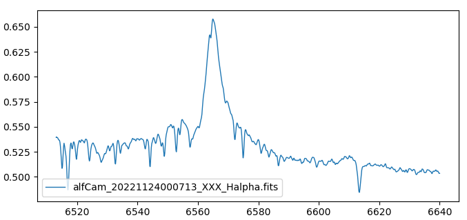
At first, a range from 6513 to 6640 is cut out of each spectrum and further work is only done with these sections. The partial spectra now contain the broad HeII line HeII6527, the extensive mountains around H-alpha and the diffuse interstellar band 6614 and lots of tellurics.
The atmospheric lines are removed from each partial spectrum as much as
possible. The removal is performed interactively and the result is simply judged by
looking at it.
Then the wavelength scale of each partial spectrum is barycentrically corrected
and freed from the Doppler shift of the radial velocity. At last a spectrum with a
velocity scale is generated with rest wave length Hα =
6562.819 Å.
The processing steps of the spectra resulting from these processes are entered in the respective headers.
Drying the Spectra
The transmission spectra of the atmosphere are computed with an resolution of around 70,000 and then convolved with a Gaussian to fit their resolution to the object spectrum. This does not fit for all wavelengths even for the small cut-out area around H alpha. The TelFit tutorial therefore proposes the SVD (Singular Value Decomposition?) method for stronger absorption lines. But I have no idea how this method works, nor how to use it. The amplitude of the transmission spectra is adjusted with an exponential function \( T(a)= T_0^a\) with amplitude \(a>0\). The wavelength scale of the original spectrum can be shifted and stretched or compressed to achieve a well dried spectrum.
An example:
The two following figures each show a zoom into the original spectrum in blue, the telluric spectrum already
adjusted in amplitude and resolution in green and the dried spectrum in orange, which is simply the quotient of blue and green.
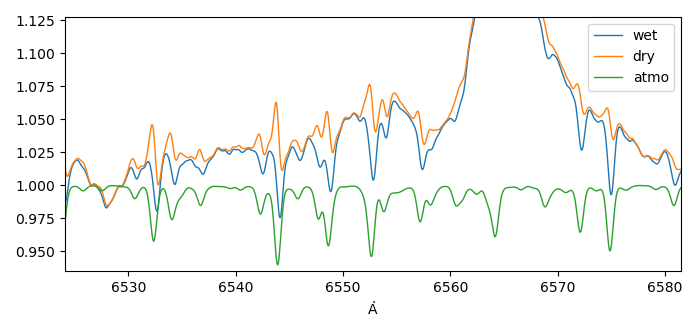
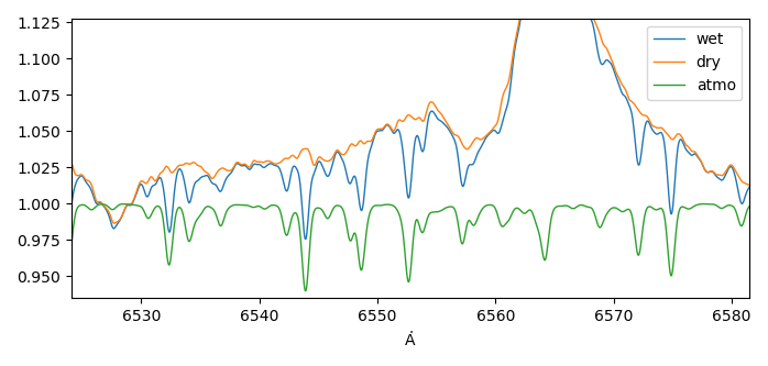
One recognizes immediately that drying can be better achieved with the transformed wavelengths.
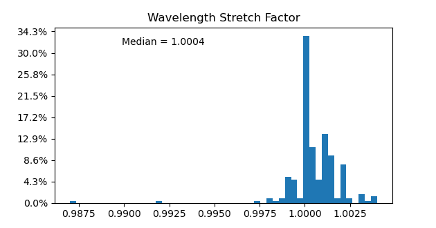
Drying the spectra thus influences the wavelengths and intensities. And that affects the reading of the equivalent width. We need to examine what errors in the values of the EQ are produced by this interactive method of drying the spectra.
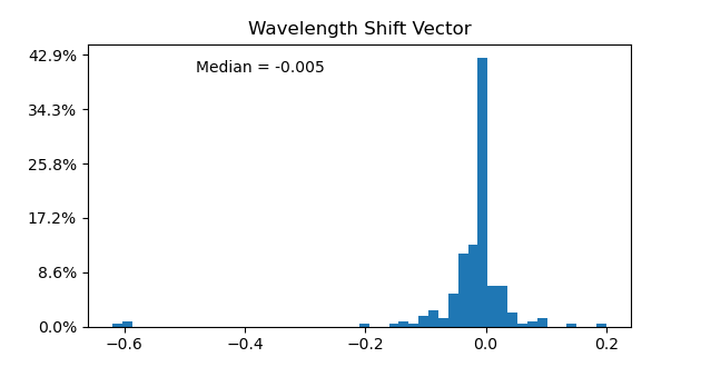
When the 232 sections around H-alpha were dried, the wavelength scales where stretched or and shifted as follows:
The shifts in wavelength were:
Shifting to the Rest Frame of alfa Cam and converting to the velocity space
After drying, there are two more steps to prepare the spectra for measurements. The wavelength is converted to the rest frame of the star and the spectrum is normalized.
For the shift into the rest frame of the star, the barycentric correction is read from the respective headers and the radial velocity of the star is subtracted from it. The new wavelengths are then \[ \lambda_{\mathrm{Star}} = ( 1 + \frac{v_{bary} - 10\,\mathrm{km/s}}{c}) \cdot \lambda_{\mathrm{Observatory}}. \] \( c = \mathrm{vacuum\ speed\ of\ light}. \)
Then the spectrum is converted to the velocity space with rest wavelength of Hα \( = \lambda_\mathrm{rest} = 6562.819\,\mathrm{Å} \) via \[v = c \cdot\frac{\lambda - \lambda_\mathrm{rest}}{\lambda_\mathrm{rest}}.\]
Normalizing the spectra
On the advice of Prof. Henrichs,
the spectra are normalized with a linear function.
This function goes through two points from the mean values of speed and intensity of two
intervals.
On the blue side [-1170 km/s, -959 km/s] and on the red side [1200 km/s, 1415 km/s].
We have reached a first resting point. Watch the video from all 232 normalized spectra.
Last modified: 2024 Feb 27